Classification of Stars
| Spectral Classification | Binary | Protostar | Brown Dwarf | White Dwarf | Red Giant | Cepheids | Neutron Star | Supergiants |


⇒ Continued From Page One
is a G2V type star
By comparing the spectral data we obtained for our star with that of stars in the G_V type category, we find a match for HD 66171 - a type G2 V. Shown below are the photo spectrum and a graph plot identfying the classification type of our star.
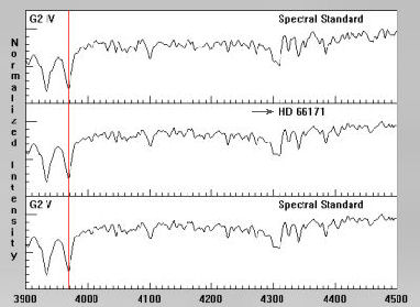
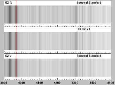
The red vertical line in the image is part of the software program used for this demostration. It is used to isolate the areas of absorption which in turn defines the element which is apparent in the spectral data. In this case the postion of the line at this measured point indicates the presence of Ca (II) or Calcium, an element seen strongest amongst type G8-K2 stars.
It should be noted that both neutral hydrogen and ionized calcium have lines very near 3970. If this line and the calcium line at 3933 are about the same strength, you can assume that the line at 3969-70 is from calcium. If the line at 3933 is much weaker, then you can assume that the line at 3969-70 is from hydrogen.
Φ = 2.512 the formulas
Lastly, we have what is called a star's "luminosity class" and it is expressed as a Roman numeral, as in " V " of our example star above. This is the energy output by the star every second, and the properties used to determine this are:
The effective temperature expressed as Teff
The size of the star which is expressed as its radius R.
Our first task is to look at a star's temperature, remembering from section II above that the hotter the star the greater the amount of radiation emitted or power output per unit of surface area. An analogy is the household light bulb and dimmer switch. At it's lowest setting the light bulb is dim and not very hot but as we rotate the dimmer switch the bulb begins to brighten, getting hotter, and this results in a greater amount of energy being emitted from it's surface area. The same principle may be applied to stars with the caveat that since the range of stellar luminosities is great our calculations need use of a constant that approximates the relationship between power and temperature. The formula used is:
l ≈ δ T4 or l is approximately equal to δ T raised to the 4th power
Where δ is the Stefan-Boltzmann constant. For a more in-depth study of δ see Wikipedia, Stefan-Boltzmann constant.
Our next step in calculating luminosity is to determine the star's surface area or radius since this relation is such that as both the unit of area and surface temperature increase so too does the emitted radiation or power output per unit of area which is what we are now calculating. The formula used for determining surface area is:
4π R2, where R is equal to the Radius of the star
Our final step at this point is to combine the two above formulas in order to calculate the star's total luminosity:
L ≈ 4π R2 δ T4
So now we have all we need in hand to calculate a star's luminosity class - except! Looking at the above calculations sort of begs the question, what is the star's radius? All the above works great if we have a star's radius to begin with but as only some hundreds of star's have had a direct measurement made of their radii the above seems to be rather acemdemic. Not so, as we are able to measure the luminosity of a star via other means - spectroscopic comparison - and through this we can actually use the above equation to determine the radius of the star, thus having in hand the information required to make our calculations. For more in-depth study and understanding see Australia Telescope Outreach and Education page entitled "The Colors of Stars".
Before ending this section, let us quickly look at Apparent Magnitude and how we calculate the difference between two stars. Remember, the higher the magnitude number the dimmer the star. So, let's say for example that Φ is a magnitude 11 star and Ω a magnitude 6 star. How many times is one star fainter than the other?
The relative magnitude formula is expressed as:
bΦ = 2.512 ( MΩ - MΦ ) bΩ
Where:
b = apparent brightness of star Φ & star Ω
M = apparent magnitude of star Φ & star Ω
and 2.512 is raised to ( MΩ - MΦ ) x bΩ
Example: Star Ω appears five magnitudes fainter than Star Φ
Solution: bΦ / bΩ = 2.512(MΩ - MΦ) → bΦ / bΩ = 2.512(5) or 100 times fainter.
Just remember, the scale is logarithmic so that a difference of 5-magnitude translates into a factor of 100x.
final word & further resources
Bear in mind that this page is not definitive, just a simple overview and as such there is much more behind the images and graphs seen here. Additionally, the science of astronomy is always, to one degreen or another, in flux as new discoveries are made and past and present theories to put to the test. Not all is 100% certain or known, including the spectral analysis of stellar objects.
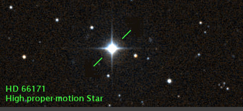
Here is another image of our star, HD 66171 obtained using the Aladin desktop applet software:
For Further Study
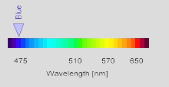
∴ Light Spectrum
A well rounded review of the color spectrum by Steve Beeson, Arizona State University
∴ The Doppler Effect
A java applet illustrating the effect with configurable parameters
∴ Color, Doppler, Red-shift
The Sloan Digital Sky Survey's SkyServer website, educational series - well done.
∴ Atomic Spectra Database
at the National Institute of Standards and Technology
∴ the Bohr model
Tutorial on Excitation by absorption of light and de-excitation by emission of light
∴ Hydorgen Emission Lines and Spectral Color
Both pages are from Georgia State University and are solid study reference of the science of spectral analysis - advance math and formulas.
∴ Christian Buil's Homepage
This site is dedicated to the use of electronic detectors in the field of astronomy and spectroscopy
∴ SBIG's new Deep Space Spectrograph
Though a retail site for amateur astronomers it provides a very good overview of the technical and working details of Spectrograph equipment.
∴ Australia Telescope Outreach and Education website
The Australia Telescope is operated as a National Facility under guidelines originally established by the Australian Science and Technology Council.
∴ Outreach Programs/Students
Links within the University of Oregon, Friends of Pine Mountain
∴ The Spectral Types of Stars
by Alan M. MacRobert, Sky & Telescope Article regarding star spectra.
I wish to acknowledge the fine efforts of the physics staff at Gettysburg College who have written a variety of educational astronomy software packages and to whom credit for the above images of the spectural "photo" and "graph" charts must go. PLEASE NOTE: Project CLEA is funded by grants from the National Science Foundation under the Division of Undergraduate Education in the program of Course and Curriculum Development, and by Gettysburg College. The intention of Project CLEA is to produce innovative teaching tools and other materials for use in an educational environment and to make this material available to astronomy educators.
Quick Nav
∴This Page
Obtaining Star Spectra
∴Next Page
Actual Spectra
∴Back To
The Star Page
∴Back To
The Main Page
footnotes
fn 1
Return to source ParagraphThe absorption features present in stellar spectra allow us to divide stars into several spectral types depending on the temperature of the star. The scheme in use today is the Harvard spectral classification scheme which was developed at Harvard college observatory in the late 1800s, and refined to its present incarnation by Annie Jump Cannon for publication in 1924. Reference source: COSMOS - The SAO Encyclopedia of Astronomy Swinburne University of Technology.
fn 2
Return to source ParagraphAtoms are neutral when they contain the same number of protons as electrons. Ionization is the physical process of converting an atom or molecule into an ion by adding or removing charged particles such as electrons or other ions. See Williams College for a study exercise entitled "Emission Lines and Central Star Temperature".
Obtaining Star Spectra
Actual Spectra
The Star Page
The Main Page
What Wavelength Goes With a Color? Atmospheric Science Data Center
Applet: Doppler Effect Visualization of the Doppler effect. The LearningOnline Network with CAPA
Classification![]()
O-B-A-F-G-K-M To find out what all those letters mean click the pic (Wikipedia).